The algorithm I want to outline in this post was developed for string clustering although it can be used for a wide range of analogous problems as well. The algorithm has several distinctive features: it does not need us to specify the number of clusters present in the dataset upfront; it does not require samples to have vector representations as long as we have some way to compute “connectedness” or distance between them; and does not make any assumptions about clusters being convex or having isotropic distributions and can detect clusters of complex shapes.
Let’s take the above characteristics one at a time.
Many common clustering algorithms such as K-means require us to specify the number of clusters we want to divide the data into ahead of time. This can indeed be useful, especially when dealing with noisy data without clear boundaries where we know there are a definite number of categories present in the data. However, there are many instances where we don’t know ahead of time how many groups there are in the data. For example, if we had a bag of M&Ms and knew ahead of time it only consisted of red, green, and blue, we could say K = 3 and cluster them. But imagine we have a bag of various colors we want to separate but we don’t know how many colors there are. In this case, we would want to use an algorithm that doesn’t need K to be stated up-front as a parameter.
Next, while most machine learning algorithms will deal with samples that are represented as vectors – i.e. if we have m samples where each is distributed over n features, we would start with an m x n matrix. Distances between various samples can be computed with an assortment of distance metrics, for example the commonly used Euclidean distance. However, on occasion, we might have samples where we are able to compute similarity or distance between them as a quantitative or categorical score (for example, connected/not connected), but where representing the samples in a vector form that can be ingested by most algorithms is either impossible or cumbersome. For example, in the case of strings containing related words or variant spellings, we might compute similarity using some metric like the Levenshtein string similarity algorithm. So, for example we might say the words “round” and “mound” have a distance or cost of 1 because we only need to switch out one letter to get from one to the other. Similarly, “book” and “back” have a distance of 2 etc – the scores being based on the number of substitutions, insertions, and deletions required. Such scores are a standard part of many Natural Language Processing tasks and offer a great deal of customizability based on problem domains. For example, if we were creating a screen typing autocorrect algorithm, we might want to treat “round” and “found” as more similar than “round” and “mound” because, even though both require The switch of a single letter, “r” and “f” are next to each other on the keyboard while “r” and “m” are far apart. Such algorithms might be really powerful and customizable ways of quantifying distances between samples, but they have no obvious vector representation that can be plugged into the usual expected matrix format. To accommodate for this, many clustering algorithms will accept square matrices (or their sparse representations) or precomputed pairwise distances.
Finally, many algorithms have expectations about the ways in which samples are distributed – for example, that they follow gaussian distributions, or are equally or symmetrically distributed along various axes. Others, mainly density based or hierarchical clustering algorithms, avoid such assumptions and can learn complex distribution shapes.
The Algorithm
The basic algorithm is quite simple. For any pair of points (p, q) we call an edge generation function e(). This function will usually be a distance function but can use any domain specific criteria to decide whether the pair of points (p, q) meet the threshold for being in the same cluster. If the criteria is met, we record an edge between the points in a network. Once all points in the sample set have been compared pairwise, we partition the resulting final network into disjointed set. Each set is a cluster of similar points. The number of sets produced is K, our number of clusters. Note that, as long as the edge function e(p, p) returns true, a node is at least connected with itself and thus we allow single item nodes.
Initialize graph g;
For a pairs (p,q) in samples set S:
If e(p,q) == True:
	Add nodes p and q to g;
	Add edge p<-->q;
Partition network g into disjointed subnetworks;
This might seem trivially simple, but it offers great versatility in many use cases. Let’s try it first with a very small subset of 10 strings selected from a 90,000 sample dataset I was working on. These are name variants of printers and publishers in the sixteenth and seventeenth centuries. They come from an immensely complex and interesting corpus of historical publishing data. Domain expertise really comes handy when devising the edge function for such a dataset. But for now let’s leave that aside and see if our algorithm can solve the clustering problem and discover that these 10 strings can be grouped into 3 clusters: 'William Caxton', 'Wyllyam Caxton', 'Wylliam Caxston', 'William Caxton', 'Wynken de Worde', 'Winkyn de Word', 'Wynkin de Word', 'Richard Pynson', 'Richard Pinson', 'Rickard Pinson'
Here’s the python code, using the networkx library.
import networkx as nx

graph = nx.Graph()
for i1,s1 in enumerate(samples):
    for i2,s2 in enumerate(samples[:i1]):
	if weighted_levenshtein(s1, s2):
	    graph.add_edge(i1, i2)
sub_g = nx.connected_components(graph)

# Let’s print out the results
for i, cluster in enumerate(sub_g):
    print(f'Cluster: {i}')
    for item_index in cluster:
	print(f'\t{samples[item_index]}')
This produces the following output:
    Cluster: 0
	Wyllyam Caxton
	Wylliam Caxston
	William Caxton
	William Caxton
    Cluster: 1
	Winkyn de Word
	Wynkin de Word
	Wynken de Worde
    Cluster: 2
	Richard Pinson
	Richard Pynson
	Rickard Pinson
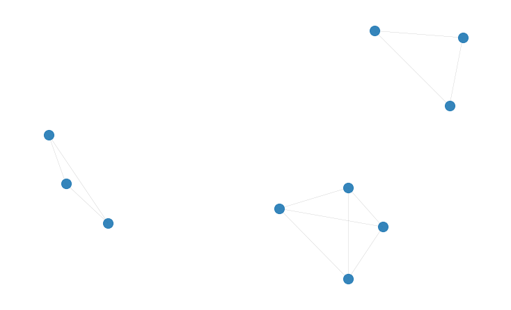
The network of 10 nodes that is generated has the following structure:
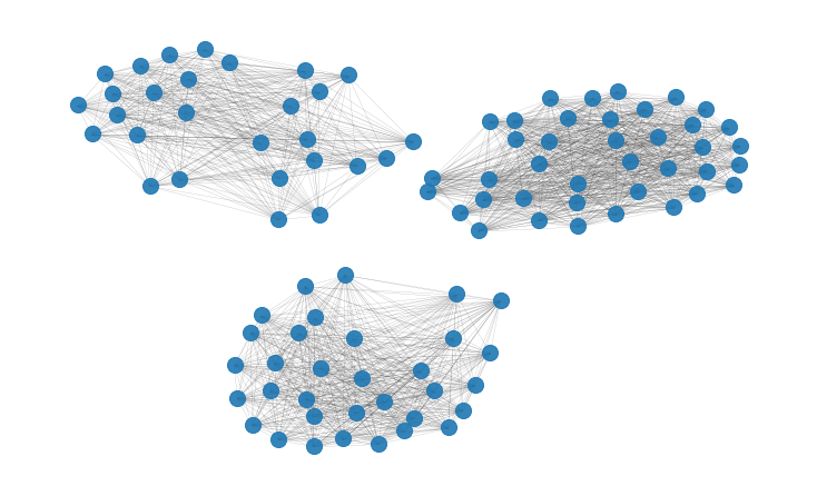
Note that even though we are calling the edge/distance function N^2/2 times within the loop, this can also be a pre-computed matrix. However, the vast majority of these calls will be able to return 0/False results really fast and only a relatively small number of calls will actually have to go through the time-consuming Levenshtein calculation (see below).
If you have experience with clustering algorithms, the above characteristics will tell you that they are shared by density based clustering algorithms such as DBSCAN and indeed the approach I am describing here has very strong similarities to density based clustering. There are a few key conceptual and implementation differences though that made this a better and faster choice for my implementation. To understand why, let’s look a little more closely at the problem.
The Problem
Here, in brief, is the problem I set out to solve. I started with a spreadsheet containing roughly 90,000 names extracted using regular expressions from a large corpus of books printed in England between 1473 and 1700. Our task is to identify unique names in this list. What looks like a trivially simple problem actually proves to be extremely complicated because spelling conventions in the sixteenth and seventeenth centuries were utterly chaotic (a fun example: Shakespeare’s name can be found with more than 80 spelling variants). Moreover, beside the usual wild spelling variations, sometimes initials are used, and sometimes Latin names – so John can show up as Iohannis. To make things even more interesting, sometimes names were shared by fathers and sons and the only way to tell them apart is from other clues such as dates when they published books and, of course, highly specialized scholarly domain knowledge. Note, finally, that we also don’t know how many total names there are – so K is unknown – and there are many names that occur only once, i.e. clusters can range in size from many hundreds in case of a prolific printer who printed many books to single-sample clusters.
This is where data preprocessing and domain knowledge becomes very important. Using some techniques I will leave for a later post, I manage to standardize the names as much as possible. Name abbreviations, variants, and initials were considered, Latin names were turned into English, common typographic practices such as using “vv” for “w” were corrected for etc. But we are still left with 90,000 widely variant names. And even though these names don’t have easy vector representations, we could certainly use Levenshtein distances as a similarity metric and generate a pairwise distance matrix. This could, theoretically, be plugged into an algorithm like scikit-learn’s implementation of DBSCAN that in the latest version now accepts a “precomputed” parameter and a pairwise distance grid in lieu of vectors.
But this would result in a grid with well over 8 billion cells and 4 billion calls to the Levenshtein distance routine (each call is quite complex and time-consuming). So again, I turned to a bit of domain knowledge to massively optimize this dataset. I used a fast prescreener to throw out name-pairs that weren’t viable reducing the set to a few hundred thousand and then used highly adjustable weights in the Levenshtein algorithm learned from my prior study of spelling variation in the period and the fact that some letters are often substituted by others (e.g. “u”/“v”, “i”/“j” etc).1 Thus, potentially N^2 distance calculations are heavily reduced by culling using computationally cheap metrics.
Now, you might notice that a network is essentially a representation of a sparse matrix where non-zero cells represent edges between nodes. Thus, the similarities between this very simple approach and density based approaches becomes clear. Originally, many of these algorithms either insisted on vector representations or complete pairwise distance grids. But current optimized implementations in the latest version of scikit-learn for example, allow for pre-computed sparse matrices that when combined with viable epsilon thresholds and a min_sample of 1, produce comparable results. But this implementation retains a significant speed advantage because the network structure only requires writing to a dictionary instead of the comparatively more complex scipy.sparse matrix implementations.
Apart from the elegance and simplicity, this implementation can be easily adapted to other uses. For example edge weights or node properties can be created while building the network, allowing further manipulation of sub-groups once clustering is completed. Thresholds can also be modified to eliminate smaller clusters as noise or to facilitate other network based machine learning algorithms. But more on such possibilities later. The current implementation – which is so trivially simple that it could be rewritten without the networkx library using pure python dictionaries in a few lines of code – is a great opportunity to explore ways of learning highly complex patterns and thinking about what a little bit of domain knowledge can do to optimize machine learning tasks.
-
Anupam Basu, “‘Ill Shapen Sounds, and False Orthography’: A Computational Approach to Early English Orthographic Variation,” in New Technologies in Medieval and Renaissance Studies, ed. Laura Estill, Michael Ullyot, and Dianne Jackaki (Arizona Center for Medieval and Renaissance Studies and Iter, 2016), 167–200. ↩